PREDIPATH : analysis of the 65x65 data
Clickable table of contents
1. Description of the data
2. Analysis of the 0/1 data: reduction of dimension
3. Analysis of the 0/1 data: prediction of the status
4. Analysis of the percentage data: reduction of dimension
5. Analysis of the percentage data: prediction of the status
6. Concluding remarks
1. Description of the data
The original data is a 65x65 matrix of percentages of identity.
The genomes, described in the file allGroups are known to be commensal or pathogenic, as shown in the following excerpt:
     ASSEMBLY_GENOME   SPECIES                                     GROUP
     GCF_000026185.1   Erwinia_tasmaniensis_Et1                    commensal
     GCF_000196615.1   Erwinia_billingiae_Eb661|Eb661              commensal
     GCF_000336255.1   Erwinia_toletana_DAPP-PG_735|DAPP-PG_735    commensal
     GCF_000745075.1   Erwinia_sp._9145|9145                       commensal
     GCF_000770305.1   Erwinia_oleae|DAPP-PG531                    commensal
     GCF_000773975.1   Erwinia_typographi|M043b                    commensal
     [...]
     GCF_002732435.1   Erwinia_amylovora|NHWL02-2                  pathogenic
     GCF_002732445.1   Erwinia_amylovora|OR1                       pathogenic
     GCF_002732485.1   Erwinia_amylovora|MANB02-1                  pathogenic
     GCF_002732505.1   Erwinia_amylovora|EA110                     pathogenic
     GCF_002803865.1   Erwinia_amylovora|E-2                       pathogenic
     GCF_002952315.1   Erwinia_pyrifoliae|EpK1                     pathogenic
The clusters are described in the file allClusters. Some clusters are shown below:
     Name       Assembly_genome
     cluster_1  argannot~~(Bla)Penicillin_Binding_Protein_Ecoli:CP002291:664439-666340:1902
     cluster_2  card~~gb|AAC75733.1|ARO:3000074|emrB
     cluster_3  card~~gb|AIL15701|ARO:3003775|Escherichia
     cluster_4  card~~gb|BAE77595.1|ARO:3003303|Escherichia
     ...
     cluster_64 vfdb_pre~~VFG043692(gi:112292717)
     cluster_65 vfdb_pre~~VFG044340(gi:292489703)
In order to better see the information, cluster names have been shortened and normalized: cluster_x becomes CL0x. The names of the genomes have been shortened too and prefixed by C for commensal or by P for pathogenic. Here is a part of the data to be analyzed, the complete file is here:
     Short-name  status     CL01 CL02 CL03 CL04   CL05 CL06 CL07 CL08 CL09 CL10   CL11 CL12   CL13  CL14   CL15

     C-0026185.1 commensal     0    0    0    0 98.095    0    0    0    0    0 95.976    0 90.984  0.00 90.783
     C-0196615.1 commensal     0    0    0    0 99.048    0    0    0    0    0 95.380    0 90.164  0.00  0.000
     C-0336255.1 commensal     0    0    0    0 98.571    0    0    0    0    0 95.746    0 90.164 90.84 90.668
     C-0745075.1 commensal     0    0    0    0 98.571    0    0    0    0    0 96.051    0  0.000  0.00 91.129
     C-0770305.1 commensal     0    0    0    0 98.571    0    0    0    0    0 96.051    0  0.000  0.00 91.129
     [...]
     P-2732445.1 pathogenic    0    0    0    0 98.571    0    0    0    0    0 96.051    0      0     0  0.000
     P-2732485.1 pathogenic    0    0    0    0 98.095    0    0    0    0    0 96.051    0      0     0  0.000
     P-2732505.1 pathogenic    0    0    0    0 98.571    0    0    0    0    0 95.976    0      0     0  0.000
     P-2803865.1 pathogenic    0    0    0    0 98.571    0    0    0    0    0 96.051    0      0     0  0.000
     P-2952315.1 pathogenic    0    0    0    0 98.571    0    0    0    0    0 95.753    0      0     0 90.323
2. Analysis of the 0/1 data: reduction of dimension
The original data have been converted to 0/1 data: if the percentage is not 0 then the value is 1. This provides a matrix of presence/absence to be analyzed.
Here is a part of the data to be analyzed, the complete file is here in text format and there in CSV format:
     Genome      status     CL01 CL02 CL03 CL04 CL05 CL06 CL07 CL08 CL09 CL10 CL11 CL12 CL13 CL14 CL15
     C-0026185.1 commensal     0    0    0    0    1    0    0    0    0    0    1    0    1    0    1
     C-0196615.1 commensal     0    0    0    0    1    0    0    0    0    0    1    0    1    0    0
     C-0336255.1 commensal     0    0    0    0    1    0    0    0    0    0    1    0    1    1    1
     C-0745075.1 commensal     0    0    0    0    1    0    0    0    0    0    1    0    0    0    1
     C-0770305.1 commensal     0    0    0    0    1    0    0    0    0    0    1    0    0    0    1
     [...]
     P-2732445.1 pathogenic    0    0    0    0    1    0    0    0    0    0    1    0    0    0    0
     P-2732485.1 pathogenic    0    0    0    0    1    0    0    0    0    0    1    0    0    0    0
     P-2732505.1 pathogenic    0    0    0    0    1    0    0    0    0    0    1    0    0    0    0
     P-2803865.1 pathogenic    0    0    0    0    1    0    0    0    0    0    1    0    0    0    0
     P-2952315.1 pathogenic    0    0    0    0    1    0    0    0    0    0    1    0    0    0    1
As one can see, some columns look similar. And in fact, some colums are equal. So we first wrote a script to remove them. Here is the result of this script:
     NB Column  Equal-to:
     01 status
     02 CL01    CL02 CL04 CL06 CL07 CL08 CL09 CL10 CL12 CL23 CL53 CL55
     04 CL03
     06 CL05
     12 CL11
     14 CL13
     15 CL14
     16 CL15
     17 CL16
     18 CL17    CL52
     19 CL18
     20 CL19    CL20
     22 CL21
     23 CL22
     25 CL24
     26 CL25
     27 CL26    CL40
     28 CL27
     29 CL28    CL29 CL31 CL32 CL38
     31 CL30
     34 CL33    CL39 CL42 CL44 CL46 CL47
     35 CL34    CL36 CL49 CL65
     36 CL35    CL50
     38 CL37
     42 CL41
     44 CL43
     46 CL45
     49 CL48
     52 CL51
     55 CL54
     57 CL56    CL57 CL58 CL59 CL60 CL61 CL62 CL63 CL64
So instead of analyzing 65 columns of 0/1 data, we have to analyze only 30 columns. Since no resulting column if constant (details not shown here), we can proceed to predict the status of the genomes.
3. Analysis of the 0/1 data: prediction of the status
The classical statistical method for the classification of two classes is called binary logistic regression. Here it fails since there is a complete separation of the data, which means there is a combination of some columns that predicts exactly the status.
We have found such a combination (probably minimal) with 4 columns:
     Coefficients Estimate Std. Error t value Pr(>|t|)
     (Intercept)  1.03273    0.02297  44.961  < 2e-16 ***
     CL41         0.96727    0.05544  17.449  < 2e-16 ***
     CL33         0.45818    0.06591   6.952 3.02e-09 ***
     CL34        -0.45818    0.08175  -5.605 5.56e-07 ***
     CL13        -0.08364    0.03574  -2.340   0.0226 *

     Signif. codes:  0 '***' 0.001 '**' 0.01 '*' 0.05 '.' 0.1 ' ' 1

     Residual standard error: 0.08739 on 60 degrees of freedom
     Multiple R-squared:  0.9697,	Adjusted R-squared:  0.9677
     F-statistic: 480.6 on 4 and 60 DF,  p-value: < 2.2e-16

     Comparing status and round(ml$fitted.values),0): perfect separation!
The minimal data needed to predict the status is then shown below:
     Details of the predictors values
     ================================

     Status 1 = commensal

                 status CL41 CL33 CL34 CL13
     C-0026185.1      1    1    0    1    1
     C-0196615.1      1    0    0    0    1
     C-0336255.1      1    0    0    0    1
     C-0745075.1      1    0    0    0    0
     C-0770305.1      1    0    0    0    0
     C-0773975.1      1    0    0    0    0
     C-1267535.1      1    0    0    0    1
     C-1267545.1      1    0    0    0    1
     C-1269445.1      1    0    0    0    1
     C-1422605.1      1    0    0    0    0
     C-1484765.1      1    0    0    0    1
     C-1517405.1      1    0    0    0    0
     C-1571305.1      1    0    0    0    1
     C-2751995.1      1    0    0    0    0
     C-2752015.1      1    0    0    0    0
     C-2752025.1      1    0    0    0    0
     C-2752055.1      1    0    0    0    0
     C-2752075.1      1    0    0    0    0
     C-2752165.1      1    0    0    0    0
     C-2752575.1      1    0    0    0    1
     C-2752595.1      1    0    0    0    0
     C-2865965.1      1    0    0    0    0
     C-2980095.1      1    0    0    0    1
     C-0068895.1      1    0    0    0    0

     Status 2 = pathogenic

                 status CL41 CL33 CL34 CL13
     P-0026985.1      2    1    1    1    0
     P-0027205.1      2    1    1    1    0
     P-0027265.1      2    1    1    1    0
     P-0091565.1      2    1    1    1    0
     P-0165815.1      2    1    1    1    0
     P-0240705.2      2    1    1    1    0
     P-0367545.1      2    1    1    1    0
     P-0367565.1      2    1    1    1    0
     P-0367585.1      2    1    1    1    0
     P-0367605.1      2    1    1    1    0
     P-0367625.1      2    1    1    1    0
     P-0367645.1      2    1    1    1    0
     P-0367665.1      2    1    1    1    0
     P-0404125.1      2    1    0    0    0
     P-0513355.1      2    1    1    1    0
     P-0513395.1      2    1    1    1    0
     P-0513415.1      2    1    1    1    0
     P-0590885.1      2    1    0    0    0
     P-0696075.1      2    1    1    1    0
     P-0975275.1      2    1    0    0    0
     P-1050515.1      2    1    0    1    0
     P-2732125.1      2    1    1    1    0
     P-2732175.1      2    1    1    1    0
     P-2732205.1      2    1    1    1    0
     P-2732215.1      2    1    1    1    0
     P-2732245.1      2    1    1    1    0
     P-2732255.1      2    1    1    1    0
     P-2732285.1      2    1    1    1    0
     P-2732295.1      2    1    1    1    0
     P-2732315.1      2    1    1    1    0
     P-2732335.1      2    1    1    1    0
     P-2732365.1      2    1    1    1    0
     P-2732385.1      2    1    1    1    0
     P-2732405.1      2    1    1    1    0
     P-2732425.1      2    1    1    1    0
     P-2732435.1      2    1    1    1    0
     P-2732445.1      2    1    1    1    0
     P-2732485.1      2    1    1    1    0
     P-2732505.1      2    1    1    1    0
     P-2803865.1      2    1    1    1    0
     P-2952315.1      2    1    1    1    0
Since these data correspond to presence/absence, a count-heatmap is probably a better way to understand these data (you can click on the image to have a better view):
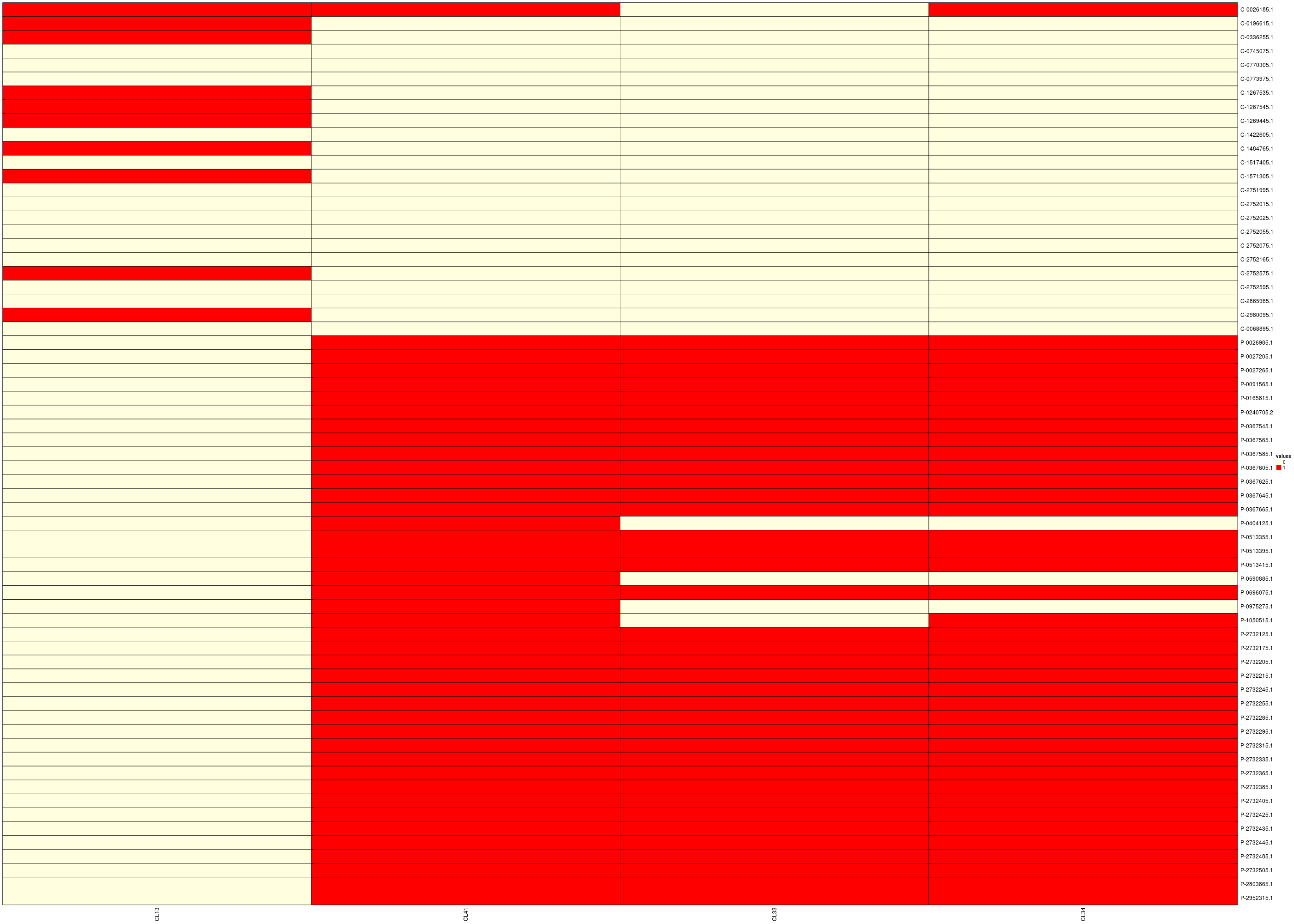
Columns: CL13 CL41 CL33 CL34; Rows: commensal then pathogenic.
Since the linear regression model is not easy to understand, the main columns used to predict the status are given below but none is specific, which means that alone none is sufficient for the prediction:
     Thresholds : presence : pct1 >=  90  %; absence: pct0 <  10  %

     no cluster is able to predict "commensal"

     6 clusters nearly allow to predict "pathogenic"

     NB   Column sum sumCommens pctCommens sumPatho pctPatho specCommens specPatho presqueCommens presquePatho
     19   CL33  37          0       0.00       37    90.24                                               YYY
     20   CL34  39          1       4.17       38    92.68                                               YYY
     21   CL35  40          1       4.17       39    95.12                                               YYY
     23   CL41  42          1       4.17       41   100.00                   YES                         YYY
     24   CL43  38          0       0.00       38    92.68                                               YYY
     25   CL45  41          1       4.17       40    97.56                                               YYY

     Details of the predicted values:
     ================================

     NB   Column sum sumCommens pctCommens sumPatho pctPatho specCommens specPatho presqueCommens presquePatho
     01   CL01   1          1       4.17        0     0.00
     02   CL03   4          4      16.67        0     0.00
     03   CL11  64         23      95.83       41   100.00                   YES            XXX          YYY
     04   CL13  10         10      41.67        0     0.00
     05   CL14  12         12      50.00        0     0.00
     06   CL15  29         21      87.50        8    19.51
     07   CL16   6          6      25.00        0     0.00
     08   CL17   2          2       8.33        0     0.00
     09   CL18  44          6      25.00       38    92.68                                               YYY
     10   CL19   1          0       0.00        1     2.44
     11   CL21  62         23      95.83       39    95.12                                  XXX          YYY
     12   CL22   1          1       4.17        0     0.00
     13   CL24  14          0       0.00       14    34.15
     14   CL25  30          0       0.00       30    73.17
     15   CL26  32          0       0.00       32    78.05
     16   CL27  30          0       0.00       30    73.17
     17   CL28  33          0       0.00       33    80.49
     18   CL30  29          0       0.00       29    70.73
     19   CL33  37          0       0.00       37    90.24                                               YYY
     20   CL34  39          1       4.17       38    92.68                                               YYY
     21   CL35  40          1       4.17       39    95.12                                               YYY
     22   CL37  34          0       0.00       34    82.93
     23   CL41  42          1       4.17       41   100.00                   YES                         YYY
     24   CL43  38          0       0.00       38    92.68                                               YYY
     25   CL45  41          1       4.17       40    97.56                                               YYY
     26   CL48  36          0       0.00       36    87.80
     27   CL51   2          0       0.00        2     4.88
     28   CL54   2          2       8.33        0     0.00
     29   CL56   1          1       4.17        0     0.00
So, roughly speaking, cluster 41 predicts nearly pathogenicity. The three other clusters are here to take care of genome C-0026185.1.
     Genome      status    predit arrondi
     C-0026185.1      1 1.4581818       1
     C-0196615.1      1 0.9490909       1
     C-0336255.1      1 0.9490909       1
     C-0745075.1      1 1.0327273       1
     C-0770305.1      1 1.0327273       1
     C-0773975.1      1 1.0327273       1
     C-1267535.1      1 0.9490909       1
     C-1267545.1      1 0.9490909       1
     C-1269445.1      1 0.9490909       1
     C-1422605.1      1 1.0327273       1
     C-1484765.1      1 0.9490909       1
     C-1517405.1      1 1.0327273       1
     C-1571305.1      1 0.9490909       1
     C-2751995.1      1 1.0327273       1
     C-2752015.1      1 1.0327273       1
     C-2752025.1      1 1.0327273       1
     C-2752055.1      1 1.0327273       1
     C-2752075.1      1 1.0327273       1
     C-2752165.1      1 1.0327273       1
     C-2752575.1      1 0.9490909       1
     C-2752595.1      1 1.0327273       1
     C-2865965.1      1 1.0327273       1
     C-2980095.1      1 0.9490909       1
     C-0068895.1      1 1.0327273       1
     P-0026985.1      2 2.0000000       2
     P-0027205.1      2 2.0000000       2
     P-0027265.1      2 2.0000000       2
     P-0091565.1      2 2.0000000       2
     P-0165815.1      2 2.0000000       2
     P-0240705.2      2 2.0000000       2
     P-0367545.1      2 2.0000000       2
     P-0367565.1      2 2.0000000       2
     P-0367585.1      2 2.0000000       2
     P-0367605.1      2 2.0000000       2
     P-0367625.1      2 2.0000000       2
     P-0367645.1      2 2.0000000       2
     P-0367665.1      2 2.0000000       2
     P-0404125.1      2 2.0000000       2
     P-0513355.1      2 2.0000000       2
     P-0513395.1      2 2.0000000       2
     P-0513415.1      2 2.0000000       2
     P-0590885.1      2 2.0000000       2
     P-0696075.1      2 2.0000000       2
     P-0975275.1      2 2.0000000       2
     P-1050515.1      2 1.5418182       2
     P-2732125.1      2 2.0000000       2
     P-2732175.1      2 2.0000000       2
     P-2732205.1      2 2.0000000       2
     P-2732215.1      2 2.0000000       2
     P-2732245.1      2 2.0000000       2
     P-2732255.1      2 2.0000000       2
     P-2732285.1      2 2.0000000       2
     P-2732295.1      2 2.0000000       2
     P-2732315.1      2 2.0000000       2
     P-2732335.1      2 2.0000000       2
     P-2732365.1      2 2.0000000       2
     P-2732385.1      2 2.0000000       2
     P-2732405.1      2 2.0000000       2
     P-2732425.1      2 2.0000000       2
     P-2732435.1      2 2.0000000       2
     P-2732445.1      2 2.0000000       2
     P-2732485.1      2 2.0000000       2
     P-2732505.1      2 2.0000000       2
     P-2803865.1      2 2.0000000       2
     P-2952315.1      2 2.0000000       2
The predictions are not robust since there are some values around 1.5; it is difficult to assign them to class 1 or 2.
4. Analysis of the percentage data: reduction of dimension
So now we are using the original data (percentages of identity). As before, we try to remove equal columns. This time, only one column can be removed:
     NB Column  Equal-to:
     01 status
     02 CL01
     03 CL02
     04 CL03
     05 CL04
     06 CL05
     07 CL06
     08 CL07
     09 CL08
     10 CL09
     11 CL10
     12 CL11
     13 CL12
     14 CL13
     15 CL14
     16 CL15
     17 CL16
     18 CL17
     19 CL18
     20 CL19    CL20
     22 CL21
     23 CL22
     24 CL23
     25 CL24
     26 CL25
     27 CL26
     28 CL27
     29 CL28
     30 CL29
     31 CL30
     32 CL31
     33 CL32
     34 CL33
     35 CL34
     36 CL35
     37 CL36
     38 CL37
     39 CL38
     40 CL39
     41 CL40
     42 CL41
     43 CL42
     44 CL43
     45 CL44
     46 CL45
     47 CL46
     48 CL47
     49 CL48
     50 CL49
     51 CL50
     52 CL51
     53 CL52
     54 CL53
     55 CL54
     56 CL55
     57 CL56
     58 CL57
     59 CL58
     60 CL59
     61 CL60
     62 CL61
     63 CL62
     64 CL63
     65 CL64
5. Analysis of the percentage data: prediction of the status
Here again the binary logistic regression fails since there is also a complete separation of the data, which means there is a combination of some columns that performs a complete separation of the data with respect to the status.
We have probably found a minimal solution with these 3 columns and their combination:
     Coefficients Estimate Std. Error t value Pr(>|t|)
     (Intercept)  1.0001358  0.0187541  53.329  < 2e-16 ***
     CL41         0.0108103  0.0005939  18.201  < 2e-16 ***
     CL33         0.0046968  0.0006854   6.853 4.14e-09 ***
     CL34        -0.0054701  0.0008640  -6.331 3.22e-08 ***

     Signif. codes:  0 '***' 0.001 '**' 0.01 '*' 0.05 '.' 0.1 ' ' 1

     Residual standard error: 0.08994 on 61 degrees of freedom
     Multiple R-squared:  0.9674,	Adjusted R-squared:  0.9658
     F-statistic: 603.5 on 3 and 61 DF,  p-value: < 2.2e-16

     Comparing status and round(ml$fitted.values),0): perfect separation!
The minimal data needed to predict the status is shown below:
     Equal values
     ============

     genome      status CL33 CL34 CL41
     C-0196615.1      1    0    0    0
     C-0336255.1      1    0    0    0
     C-0745075.1      1    0    0    0
     ...
     P-2732485.1      2  100  100  100
     P-2732505.1      2  100  100  100
     P-2803865.1      2  100  100  100

     Unequal values
     ==============

     genome      status CL33 CL34 CL41
     C-0026185.1      1    0   97   94
     P-0026985.1      2   92   98   99
     P-0027265.1      2   92   98   99
     P-0165815.1      2   92   98   99
     P-0404125.1      2    0    0   92
     P-0590885.1      2    0    0   94
     P-0975275.1      2    0    0   92
     P-1050515.1      2    0   94   94
     P-2952315.1      2   92   98   99
Here are the predicted values:
     genome      status    predicted rounded
     C-0026185.1      1    1.490340       1
     C-0196615.1      1    1.000136       1
     C-0336255.1      1    1.000136       1
     C-0745075.1      1    1.000136       1
     C-0770305.1      1    1.000136       1
     C-0773975.1      1    1.000136       1
     C-1267535.1      1    1.000136       1
     C-1267545.1      1    1.000136       1
     C-1269445.1      1    1.000136       1
     C-1422605.1      1    1.000136       1
     C-1484765.1      1    1.000136       1
     C-1517405.1      1    1.000136       1
     C-1571305.1      1    1.000136       1
     C-2751995.1      1    1.000136       1
     C-2752015.1      1    1.000136       1
     C-2752025.1      1    1.000136       1
     C-2752055.1      1    1.000136       1
     C-2752075.1      1    1.000136       1
     C-2752165.1      1    1.000136       1
     C-2752575.1      1    1.000136       1
     C-2752595.1      1    1.000136       1
     C-2865965.1      1    1.000136       1
     C-2980095.1      1    1.000136       1
     C-0068895.1      1    1.000136       1
     P-0026985.1      2    1.965778       2
     P-0027205.1      2    2.003826       2
     P-0027265.1      2    1.965778       2
     P-0091565.1      2    2.003826       2
     P-0165815.1      2    1.965778       2
     P-0240705.2      2    2.003826       2
     P-0367545.1      2    2.003826       2
     P-0367565.1      2    2.003826       2
     P-0367585.1      2    2.003826       2
     P-0367605.1      2    2.003826       2
     P-0367625.1      2    2.003826       2
     P-0367645.1      2    2.003826       2
     P-0367665.1      2    2.003826       2
     P-0404125.1      2    1.999958       2
     P-0513355.1      2    2.003826       2
     P-0513395.1      2    2.003826       2
     P-0513415.1      2    2.003826       2
     P-0590885.1      2    2.014876       2
     P-0696075.1      2    2.003826       2
     P-0975275.1      2    1.999958       2
     P-1050515.1      2    1.502364       2
     P-2732125.1      2    2.003826       2
     P-2732175.1      2    2.003826       2
     P-2732205.1      2    2.003826       2
     P-2732215.1      2    2.003826       2
     P-2732245.1      2    2.003826       2
     P-2732255.1      2    2.003826       2
     P-2732285.1      2    2.003826       2
     P-2732295.1      2    2.003826       2
     P-2732315.1      2    2.003826       2
     P-2732335.1      2    2.003826       2
     P-2732365.1      2    2.003826       2
     P-2732385.1      2    2.003826       2
     P-2732405.1      2    2.003826       2
     P-2732425.1      2    2.003826       2
     P-2732435.1      2    2.003826       2
     P-2732445.1      2    2.003826       2
     P-2732485.1      2    2.003826       2
     P-2732505.1      2    2.003826       2
     P-2803865.1      2    2.003826       2
     P-2952315.1      2    1.965778       2
Here also a count-heatmap is probably a better way to understand these data (you can click on the image to have a better view):
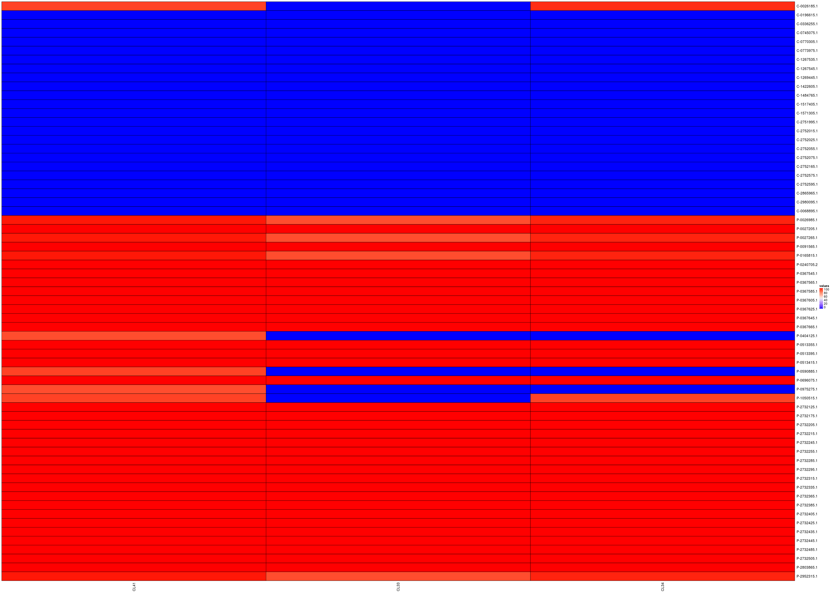
Columns: CL41 CL33 CL34; Rows: commensal then pathogenic.
So, as previously, cluster 41, named vfdb_pre~~VFG041501(gi:292487026), is nearly a predictor of pathogenicity since all pathogenic genomes have a non zero value for this cluster and all commensal genomes are null for this cluster except the genome named GCF_000026185.1 Erwinia_tasmaniensis_Et.
As before the predictions are not robust since again there are some values around 1.5; it is also difficult to assign them to class 1 or 2.
6. Concluding remarks
Though we have found some predictors for the status, the solution is not robust since one genomes can change it all.
If it was possible to ignore genome C-0026185.1 the predictor for pathogenicity would be exactly the presence of cluster 41, identified as vfdb_pre~~VFG041501(gi:292487026).
One has to think, using the 0/1 matrix, of the clusters equal to the predictors CL33 and CL34.
In order to get a robust classification, we have to think of a new strategy:
-
We can remove genome named GCF_000026185.1 Erwinia_tasmaniensis_Et so pathogenicity can be considered as equal to CL41 greater than 90.
-
We can analyze the real status of genome named GCF_000026185.1 Erwinia_tasmaniensis_Et for it may be pathogenic with a bad annotation.
-
We can decide to add more data to be sure of the information.
-
We can refine pathogenicity using more than two levels.
Code-source de cette page.
|  Retour à la page principale de
(gH)
Retour à la page principale de
(gH)